Calculator to compute the average molecular weight of a gas mixture

Unlock the Secrets of Gas Mixtures: Calculate Average Molecular Weight with Our Free Tool

Are you working with gas mixtures and need a quick, reliable way to determine their average molecular weight? Understanding the average molecular weight of a gas mixture is crucial in many scientific and engineering applications, from chemical reactions to industrial processes. This value, a weighted average of the molecular weights of all components, helps you predict a mixture's behavior and properties. Our free online calculator makes this calculation easy and accurate, saving you time and effort.

Whether you're a student learning about gas laws, a chemist working in a lab, or an engineer designing industrial equipment, our average molecular weight calculator provides you with an indispensable tool. It can help you:

• Quickly calculate the average molecular weight for complex gas mixtures.
• Understand how the composition of a gas mixture affects its overall molecular weight.
• Verify your calculations for accuracy and avoid costly errors.
• Save time and effort compared to manual calculations.
• Explore various scenarios by dynamically adding or removing the components of a mixture.

Average Molecular Weight Calculator

Enter the mole percentage and molecular weight of each component.

Explore different combinations of gases and see how the average molecular weight changes. Understanding average molecular weights is an important step towards mastering the gas laws and applying them to various scientific problems. Use this free tool as an exploration tool to experiment with mixtures of different compositions. This tool is a powerful asset in studying and understanding the properties of gas mixtures. For those interested in learning more, we encourage further reading on the gas laws and chemical thermodynamics.

Theoretical Background 

The average molecular weight of a gas mixture is calculated using the following formula: 

MW_avg = ∑ (y_i × MW_i) 

 where:

• MW_avg is the average molecular weight of the gas mixture
• y_i is the mole fraction of component i
• MW_i is the molecular weight of component i

Relation to Properties and Component Variables 

• Density: The average molecular weight affects the density of the gas mixture. 
• Viscosity: The average molecular weight influences the viscosity of the gas mixture. 
• Thermal conductivity: The average molecular weight impacts the thermal conductivity of the gas mixture. 
• Component mole fractions: The average molecular weight is calculated from the mole fractions of the individual components. 

Applications

 

• Distillation: Average molecular weight is essential in designing and operating distillation columns. 
• Mass transfer: Average molecular weight affects the mass transfer rates in gas-liquid systems.
• Thermodynamics: Average molecular weight is used in thermodynamic calculations, such as computing the entropy and enthalpy of gas mixtures.

We provide a MATLAB script designed to calculate the average molecular weight of various gas mixtures. The script defines a set of predefined gas mixtures, including flue gas, coke oven gas, bio gas, natural gas, and air. Each gas mixture is represented by its composition, which is a set of mole fractions of its constituent components.

gas_mixtures = {

    'Flue Gas', [0.03, 0.12, 0.05, 0.80];  % CO2, O2, H2O, N2

    'Coke Oven Gas', [0.03, 0.05, 0.25, 0.67];  % CO2, O2, CO, H2

    'Bio Gas', [0.30, 0.20, 0.50, 0];  % CO2, CH4, H2, N2 (assuming no N2)

    'Natural Gas', [0.01, 0, 0, 0.99];  % CO2, O2, H2O, CH4

    'Air', [0.03, 0.21, 0, 0.76];  % CO2, O2, H2O, N2

};

% Define molecular weights

molecular_weights = [44.01, 32.00, 18.02, 28.01];  % CO2, O2, H2O, N2/CH4

% Calculate average molecular weights

average_molecular_weights = zeros(size(gas_mixtures, 1), 1);

for i = 1:size(gas_mixtures, 1)

    composition = gas_mixtures{i, 2};

    average_molecular_weights(i) = sum(composition .* molecular_weights);

end

% Display results

for i = 1:size(gas_mixtures, 1)

    fprintf('%s: %.2f g/mol\n', gas_mixtures{i, 1}, average_molecular_weights(i));

end

The script then calculates the average molecular weight of each gas mixture by multiplying the mole fraction of each component by its molecular weight and summing the results. The average molecular weights are then displayed for each gas mixture.

Flue Gas: 28.47 g/mol

Coke Oven Gas: 26.19 g/mol 

Bio Gas: 28.61 g/mol 

Natural Gas: 28.17 g/mol 

Air: 29.33 g/mol 

Average molecular weights of various gas mixtures

MATLAB Simulation Experiment from Basics to Process Dynamic Simulation Using Simulink

Open-loop simulation:

(1) open Simulink by double-clicking Simulink from the menu of the matlab command window.

(2) This opens the Simulink window and from the menu bar select a new file.

(3) A new file of Simulink is opened and it is named (default) as untitled.mdl. All Simulink files have mdl extension.

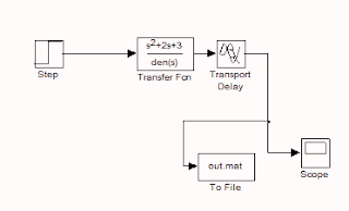
(4) From the Simulink library open ‘continuous’ icon. The transfer function is given in the continuous library as 1/(s+1) and transport delay is also given in continuous library. Drag the transfer function and drop in the new Simulink file. Similarly, drag and drop transport delay also.

(5) Now open Simulink library icon ‘sources’. Drag step function from it and drop in a new file.

(6) Now open Simulink library icon ‘sinks’. From ‘sinks’ drag and drop ‘scope’ and ‘untitled mat’ into the Simulink file.

(7) Now connect all these blocks by using a left click of the mouse.. If the existing line between two blocks is to be joined to another block, then use right click of the mouse.

(8) Once the block diagram is over, change the output file name from untitled mat to your pet name by double-clicking it. The default output variable is an in that file and you can change it according to your problem. Set the sample time as 0.01 which means the data is stored for every 0.01 sec. press ok.

(9) Double click the transfer function. Numerator and denominator are to be given according to your problem in the decreasing order of s. click ok

(10) Double click steps icon and give the time at which the step change is to be given to the process and initial and final value for the step is to be given and sample time is same as 0.01.

(11) Double click the transport delay and set the delay of the process as per the problem at hand and press ok

(12) Save this file with a name.mdl

(13) To simulate this block diagram, open simulation in the menu bar and select simulation parameters in it. Give the stop according to your problem and press ok.

(14) To simulate the block diagram press solid forward arrow symbol in the menu bar.

(15) Once the simulation is over, open Matlab command window and load the output file using the command load.

(16) Example: >>load out.mat

(17) To plot the step response use the command >>plot(y(1,:),y(2,:))[y is the output variable name which is used instead of default ans). This means the first row of y which is a time vector is plotted against the response vector (2 row of y). Then label the axis using xlabel and ylabel commands.

The open-loop block diagram is given below

Open loop

Closed loop simulation:

For closed loop simulation, additional blocks of PID controller and a summation block are required. The additional step function is required for regulatory or load problem,

PID controller is available in Simulink extras of the simulink library. Double-clicking Simulink extras, select additional linear. PID controller is available in that. Drag and drop PID into an untitled Simulink file along with transfer function, step, to file, scope.

Drag and drop sum block from Math of Simulink library and we need two of them for the simulation of the servo (setpoint change) and the regulatory problem (load change).

Connect the blocks as shown in the figure given below.

Closed loop

To give PID values, double-click PID block. In Proportional give kc value, integral give kc/I and derivative give kc*I value. Click ok.

For example, consider a transfer function model of a process as. Conduct closed-loop simulation for servo and a regulatory problem for a unit set to change in setpoint at time=0 and a unit step change in load at time=100.

(a) P controller with kc=1.9

(b) PI controller with kc=1.7 and I=14.3s

(c) PID controller with kc=1.6, I=12.5s,D=0.5s

To simulate for both servo and regulatory simultaneously, double-click step (setpoint input) and time are set equal to zero and the initial value is zero and the final value is 1. sample time is 0.01. Now double click step (load input) and time are set equal to 100 (it is the time at which servo response reaches to 1) and initial value zero and final value 1. The sample time is 0.01. i.e. Load is initiated after 100s.

Simulation time is fixed by selecting simulation parameters in the menu bar. The simulation time should be around 200 to stabilize the regulatory response as the load step is initiated at 100.

Once the simulation is over, load the result file in the Matlab command window.
>> load result.mat
>> figure,plot(y(1,:),y(2,:),'k')
>> xlabel 'time'
>> ylabel 'response'
Here the output file name is result.mat and the variable name is y. The first row of y stores time and second row of y stores response. The figures generated are

P controller

In PID block substitute P parameters as kc, 0I and 0 for proportional, integral and derivative time locations.
Simulate and then load the file in matlab command window and plot as shown below.
>> load result.mat
>> figure,plot(y(1,:),y(2,:))
>> xlabel 'time'
>> ylabel 'response'

P controller response

PI controller

In PID block substitute PI parameters as kc, kc/I and 0 for proportional, integral and derivative time locations.
Simulate and then load the file in matlab command window and plot as shown below.
>> load result.mat
>> figure,plot(y(1,:),y(2,:),'k')
>> xlabel 'time'
>> ylabel 'response'

PI controller response

PID controller

In PID block substitute PID parameters as kc, kc/I and kc*D for proportional, integral and derivative time locations.

Simulate and then load the file in matlab command window and plot as shown below.
>> load result.mat
>> figure,plot(y(1,:),y(2,:),'k')
>> xlabel 'time'
>> ylabel 'response'

PID controller response

Hydrogen Production and Hydrogen Storage Techniques

Hydrogen, a clean and efficient fuel, is revolutionizing the way we think about energy consumption. With its incredible energy density and zero-emission combustion byproduct - water - hydrogen is poised to play a vital role in reducing our reliance on fossil fuels and mitigating climate change.

The benefits of hydrogen are numerous. Not only does it produce an enormous amount of energy during combustion, but it also increases the economy and efficiency of machines. However, despite its potential, the availability and production technologies for hydrogen are still in their infancy.

One of the primary challenges facing hydrogen production is the source and raw material required. Fossil fuels, which contain high concentrations of hydrogen, are not a viable option as they perpetuate the cycle of pollution. Water, on the other hand, is an abundant resource that can be used to produce hydrogen. However, splitting water into hydrogen and oxygen requires energy, which is a significant hurdle.

The process of splitting water into hydrogen and oxygen is known as electrolysis. The mathematical relation involved in electrolysis is as follows:

2H2O → 2H2 + O2

where 2H2O represents two molecules of water, 2H2 represents two molecules of hydrogen, and O2 represents one molecule of oxygen.

The energy required to split water into hydrogen and oxygen can be calculated using the following equation:

ΔG = ΔH - TΔS

where ΔG is the Gibbs free energy, ΔH is the enthalpy change, T is the temperature in Kelvin, and ΔS is the entropy change.

As research continues to advance, we can expect to see more efficient and cost-effective methods for producing hydrogen from water. This will be a crucial step towards transitioning to a clean and sustainable energy future.

Hydrogen Production Techniques

1. Silicon Chip-Based Microreactor by Methanol Reforming

Methanol reforming is a process that converts methanol into hydrogen and carbon dioxide using a catalyst. This process can be performed in a silicon chip-based microreactor.

2. Water Splitting by Solar Energy Using Thermochemical Cycle or Water Electrolysis

Water splitting is a process that separates water into hydrogen and oxygen using energy from the sun. This can be done through a thermochemical cycle or water electrolysis.

3. Photoelectrolysis

Photoelectrolysis is a process that uses light to split water into hydrogen and oxygen. This process uses a photoelectrode to convert light energy into chemical energy.

4. Reforming of Natural Gas

Natural gas reforming is a process that converts natural gas into hydrogen and carbon dioxide using a catalyst.

5. Gasification of Coal and Biomass

Gasification is a process that converts coal or biomass into a gas mixture containing hydrogen, carbon monoxide, and carbon dioxide.

6. Photo-Biological Method with High-Temperature Decompositions

The photo-biological method uses microorganisms to produce hydrogen through photosynthesis. High-temperature decompositions can also be used to produce hydrogen from biomass.

7. Hydrocarbon Reforming

Hydrocarbon reforming is a process that converts hydrocarbons into hydrogen and carbon dioxide using a catalyst.

8. Ammonia Cracking

Ammonia cracking is a process that converts ammonia into hydrogen and nitrogen using a catalyst.

9. Pyrolysis

Pyrolysis is a process that converts biomass into a gas mixture containing hydrogen, carbon monoxide, and carbon dioxide through thermal decomposition.

10. Aqueous Reforming

Aqueous reforming is a process that converts biomass or organic compounds into hydrogen and carbon dioxide using a catalyst in an aqueous solution.

11. High-Temperature Electrolysis

High-temperature electrolysis is a process that splits water into hydrogen and oxygen using electricity at high temperatures.

12. Photo-Electrolysis (Photolysis)

Photo-electrolysis, also known as photolysis, is a process that uses light to split water into hydrogen and oxygen.

13. Photo-Biological Production (Biophotolysis)

Photo-biological production, also known as biophotolysis, is a process that uses microorganisms to produce hydrogen through photosynthesis.

All above technologies depend on the raw material used for the production of hydrogen, the mostly known feedstocks and process dependents are Algae, Gas, Oil, Wood, Coal, biomass and Power.

Efficiency metrics of the 13 hydrogen production techniques:

Hydrogen production techniques

 

Technique	Efficiency Range (%)	Energy Efficiency (%)	Cost-Effectiveness ($/kg H2)	Environmental Impact (g CO2/kg H2)
Silicon Chip-Based Microreactor by Methanol Reforming	70-90	80	2-3	100-200
Water Splitting by Solar Energy Using Thermochemical Cycle	10-20	15	5-6	50-100
Photoelectrolysis	10-20	12	6-7	40-80
Reforming of Natural Gas	70-90	85	1-2	150-300
Gasification of Coal and Biomass	40-60	50	3-4	200-400
Photo-Biological Method with High-Temperature Decompositions	10-20	12	6-7	40-80
Hydrocarbon Reforming	70-90	80	2-3	100-200
Ammonia Cracking	50-70	60	2-3	80-150
Pyrolysis	40-60	50	3-4	200-400
Aqueous Reforming	50-70	60	2-3	80-150
High-Temperature Electrolysis	70-90	80	2-3	100-200
Photo-Electrolysis (Photolysis)	10-20	12	6-7	40-80
Photo-Biological Production (Biophotolysis)	10-20	12	6-7	40-80

a) Hydrogen from NG

We have three chemical production processes

1. Steam reforming

      CH4 + H2O + heat → CO + 3H2 ( Primary reforming reaction) 
      CO + H2O → CO2 + H2 + heat ( water-gas shift reaction)

Mathematical Model: 

Assumptions:

• The reactions are carried out in a plug-flow reactor.
• The system is at steady state.
• The reactions are irreversible.
• The heat of reaction is negligible.

Model Equations:

 

Mass balance for CH₄:

 

• ∂(F_CH4)/∂z = -r₁ * A

Mass balance for H₂O:

 

• ∂(F_H2O)/∂z = -r₁ * A - r₂ * A

 

Mass balance for H₂:

 

• ∂(FH₂)/∂z = 3 * r₁ * A + r₂ * A

 

Mass balance for CO:

 

• ∂(F_CO)/∂z = r₁ * A - r₂ * A

 

Mass balance for CO2:

 

• ∂(F_CO2)/∂z = r₂ * A

 

Reaction Rates:

 

Steam reforming reaction rate:

 

• r₁ = k₁ * (F_CH4 / F_tot) * (F_H2O / F_tot)

 

Water-gas shift reaction rate:

 

• r₂ = k₂ * (F_CO / F_tot) * (F_H2O / F_tot)

Boundary Conditions:

 

Inlet conditions:

 

• F_CH4(0) = F_CH4_in
• F_H2O(0) = F_H2O_in
• F_H2(0) = 0
• F_CO(0) = 0
• F_CO2(0) = 0

 

Outlet conditions:

 

• ∂(F_CH4)/∂z(L) = 0
• ∂(F_H2O)/∂z(L) = 0
• ∂(F_H2)/∂z(L) = 0
• ∂(F_CO)/∂z(L) = 0
• ∂(F_CO2)/∂z(L) = 0

 

Parameters:

 

• k₁: steam reforming reaction rate constant
• k₂: water-gas shift reaction rate constant
• A: cross-sectional area of the reactor
• L: length of the reactor
• F_tot: total molar flow rate
• F_CH4_in: inlet molar flow rate of CH4
• F_H2O_in: inlet molar flow rate of H2O

This model can be solved using numerical methods, such as the method of lines or finite difference methods, to obtain the profiles of the species concentrations along the reactor length.

Here, we will use the finite difference method to discretize the model equations and solve them using MATLAB.

% Define the parameters

k1 = 0.1;  % steam reforming reaction rate constant

k2 = 0.05;  % water-gas shift reaction rate constant

A = 1;  % cross-sectional area of the reactor

L = 10;  % length of the reactor

Ftot = 1;  % total molar flow rate

FCH4_in = 0.5;  % inlet molar flow rate of CH4

FH2O_in = 0.5;  % inlet molar flow rate of H2O

% Define the grid size

N = 100;

dz = L / (N - 1);

z = linspace(0, L, N);

% Initialize the arrays to store the solution

FCH4 = zeros(N, 1);

FH2O = zeros(N, 1);

FH2 = zeros(N, 1);

FCO = zeros(N, 1);

FCO2 = zeros(N, 1);

% Set the inlet conditions

FCH4(1) = FCH4_in;

FH2O(1) = FH2O_in;

FH2(1) = 0;

FCO(1) = 0;

FCO2(1) = 0;

% Solve the model equations using finite difference method

for i = 2:N

    FCH4(i) = FCH4(i-1) - k1 * (FCH4(i-1) / Ftot) * (FH2O(i-1) / Ftot) * dz;

    FH2O(i) = FH2O(i-1) - k1 * (FCH4(i-1) / Ftot) * (FH2O(i-1) / Ftot) * dz - k2 * (FCO(i-1) / Ftot) * (FH2O(i-1) / Ftot) * dz;

    FH2(i) = FH2(i-1) + 3 * k1 * (FCH4(i-1) / Ftot) * (FH2O(i-1) / Ftot) * dz + k2 * (FCO(i-1) / Ftot) * (FH2O(i-1) / Ftot) * dz;

    FCO(i) = FCO(i-1) + k1 * (FCH4(i-1) / Ftot) * (FH2O(i-1) / Ftot) * dz - k2 * (FCO(i-1) / Ftot) * (FH2O(i-1) / Ftot) * dz;

    FCO2(i) = FCO2(i-1) + k2 * (FCO(i-1) / Ftot) * (FH2O(i-1) / Ftot) * dz;

end

% Plot the results

figure;

plot(z, FCH4, 'b-', z, FH2O, 'r-', z, FH2, 'g-', z, FCO, 'c-', z, FCO2, 'm-');

xlabel('Reactor Length (m)');

ylabel('Molar Flow Rate (mol/s)');

legend('CH4', 'H2O', 'H2', 'CO', 'CO2');

This code solves the model equations using the finite difference method and plots the molar flow rates of the species along the reactor length. The results show the conversion of CH4 and H2O to H2, CO, and CO2 along the reactor length.

Conversion of Natural gas to Hydrogen along the Plug Reactor

2. Partial oxidation
      CH4 + 1 / 2O2 → CO + 2H2 + heat
3. Auto thermal reforming the above two methods are used simultaneously.

b) Hydrogen from Coal

By coal gasification in a fixed bed or fluidized bed gasifier hydrogen can be produced
       C(s) + H2O + heat → CO + H2

c) Hydrogen production from water by splitting

       H2O + electricity → H2 + 1 / 2O

d) Alkaline electrolysis cell

Alkaline electrolysis

        Electrolyte: 4H2O ↔ 4H+ + 4OH–
        Cathode: 4 H+ + 4e–↔2H2
        Anode: 4OH– ↔ O2 + 2H2O + 4e–
        Sum: 2H2O ↔ O2 + 2H2

e) Polymer electrolyte membrane (PEM) electrolysis

        Anode: H2O→ 1 / 2O2 + 2 H+ + 2e–
        Cathode: 2H+ + 2e–→ H2

Photosynthesis: 2H2O → 4H+ + 4e– + O2
Hydrogen Production: 4H+ + 4e–→ 2H2

f) High-temperature decomposition

Thermo-chemical water splitting
(850 °C):          H2SO4 ↔ SO2 + H2O + 1 / 2
(120 °C):           I2 + SO2 + 2H2O → H2SO4 +
(450 °C):         2HI → I2 + H2
SUM:              H2O → H2 + 1 / 2O2

Hydrogen storage in solid form:

• Using microporous metal-organic materials
• Carbon nanotubes and graphite nanofibers
• Platinum and palladium nonporous films
• Using boron nitride nanotubes

Hydrogen storage in liquid form:

• Composite tanks
• Glass microspheres
• Cryogenic liquid hydrogen (LH2)
• NaBH4 solutions: NaBH4 (l) + 2H2O (l) → 4H2 (g) + NaBO2 (s) (ideal reaction)
• Rechargeable organic liquids